Advanced SQL Query Techniques for Data Engineers

SQL is considered the lingua franca for structured data. Database pioneer Michael Stonebraker has described SQL as “intergalactic data-speak,” referencing the fact that it is a universal language for data. 

SQL is involved in almost every aspect of data engineering, from moving data around with ETL to creating and maintaining complex data models. Thus, data engineers often require deep-level expertise in SQL. Unfortunately, despite being an easy skill to pick up, SQL is difficult to master. 

This article will provide advanced SQL techniques for improving query efficiency and system performance. We will also present practical examples to show how these techniques can be applied to overcome common challenges in data engineering. 

What Makes an SQL Query Advanced?

The term "advanced SQL query" refers to complex SQL queries that go beyond the basic functionalities of manipulating databases. Advanced SQL is not only about executing complex queries but also optimizing them for efficiency and reliability across different database systems. 

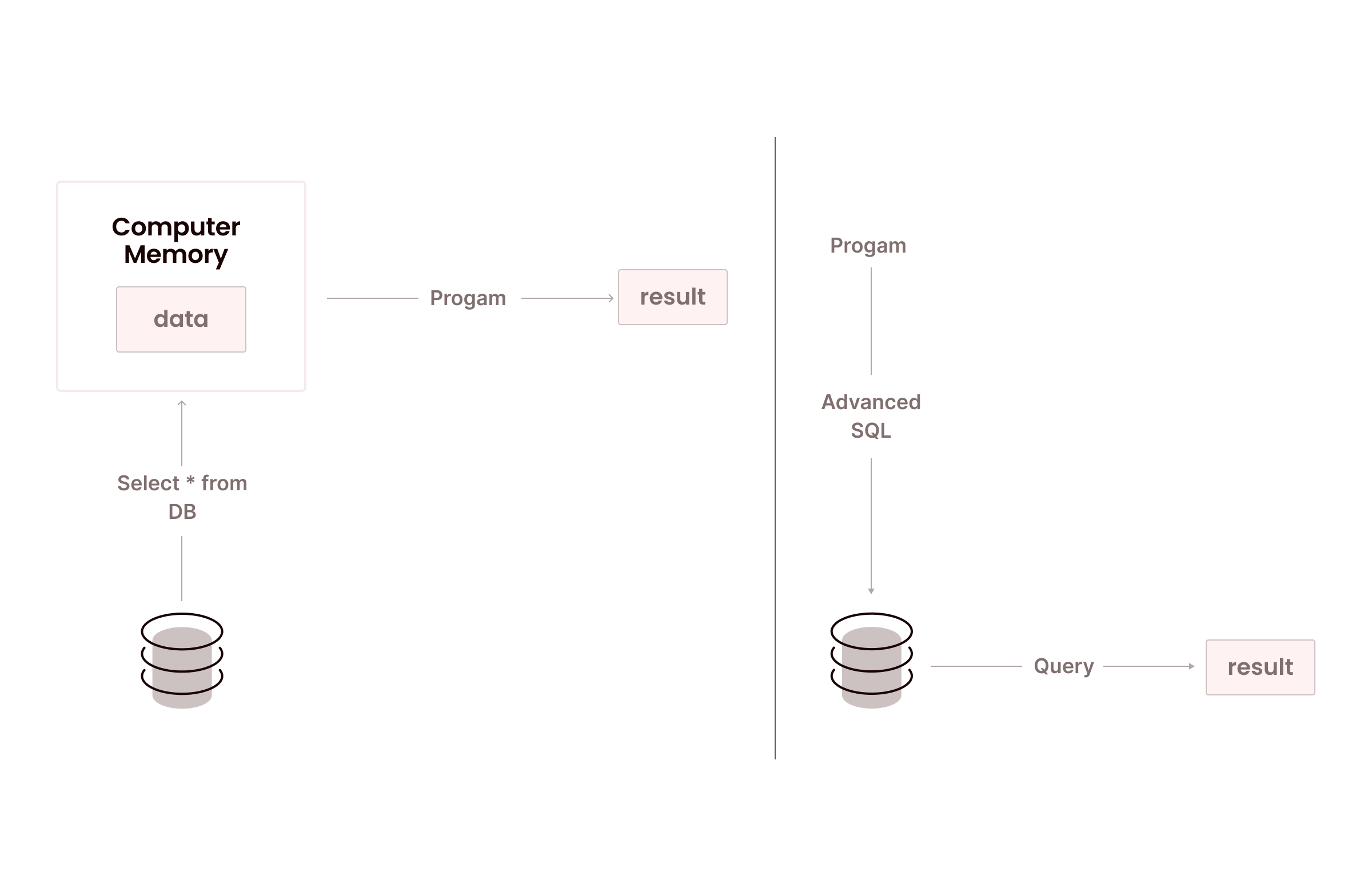
As shown in Figure 1, normal SQL moves entire tables out of the database into the application and then performs in-heap computation to obtain the result. Advanced SQL moves the computation close to the data. This level of SQL includes:

• SQL window functions to extend SQL's capabilities in analytics
• Recursive data exploration to enhance the handling of hierarchical and recursive data
• Optimization to boost the performance and efficiency of database queries
• Complex data transformations to manage intricate data reshaping and integration tasks effectively
• Tuning to boost SQL ops performance and efficiency
• Advanced error handling and debugging for higher reliability and accuracy of SQL scripts

SQL Window Functions

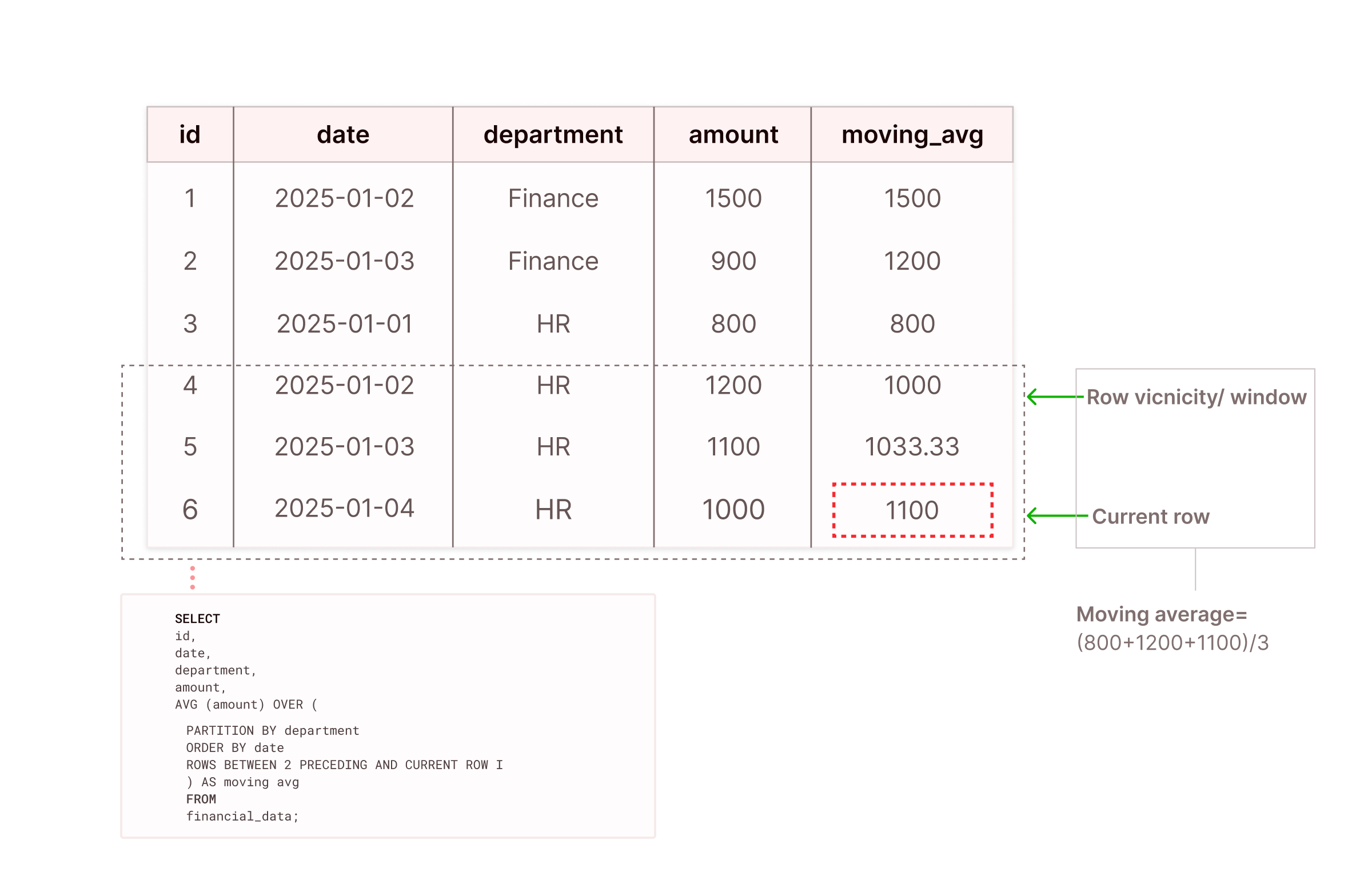
SQL window functions are expressive features of modern SQL designed to handle complex computations. Unlike other SQL functions, window functions can take row vicinity as the input and generate a single value. 

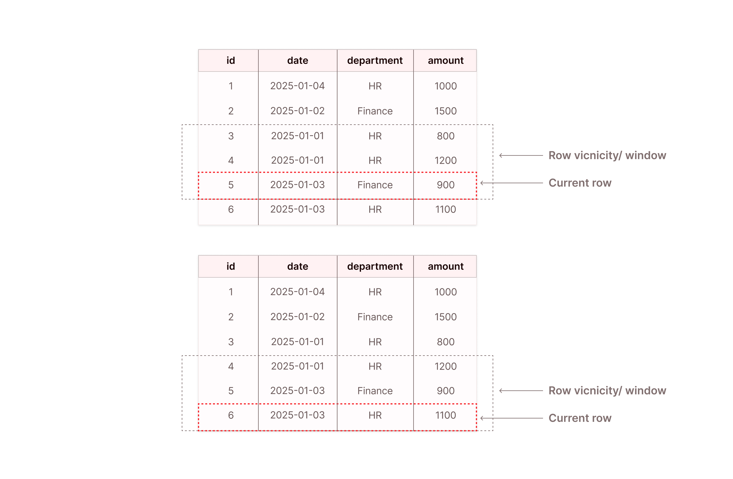
Row vicinity can be simplified as the visibility beyond the current row of execution (i.e., some rows before and some rows after the current row). When the current row changes, the row vicinity window slides with it, as seen in Figure 2 below. 

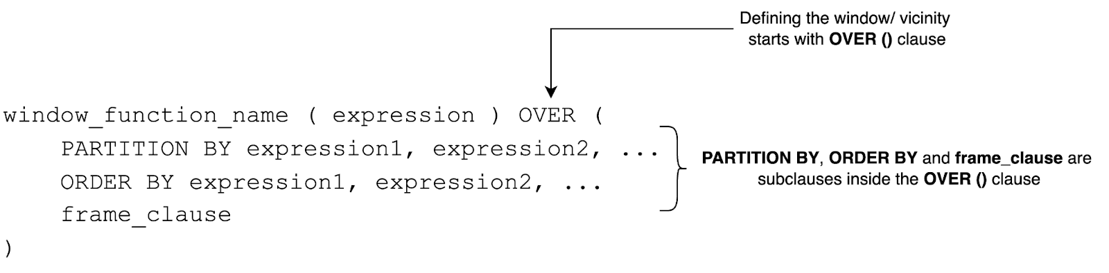
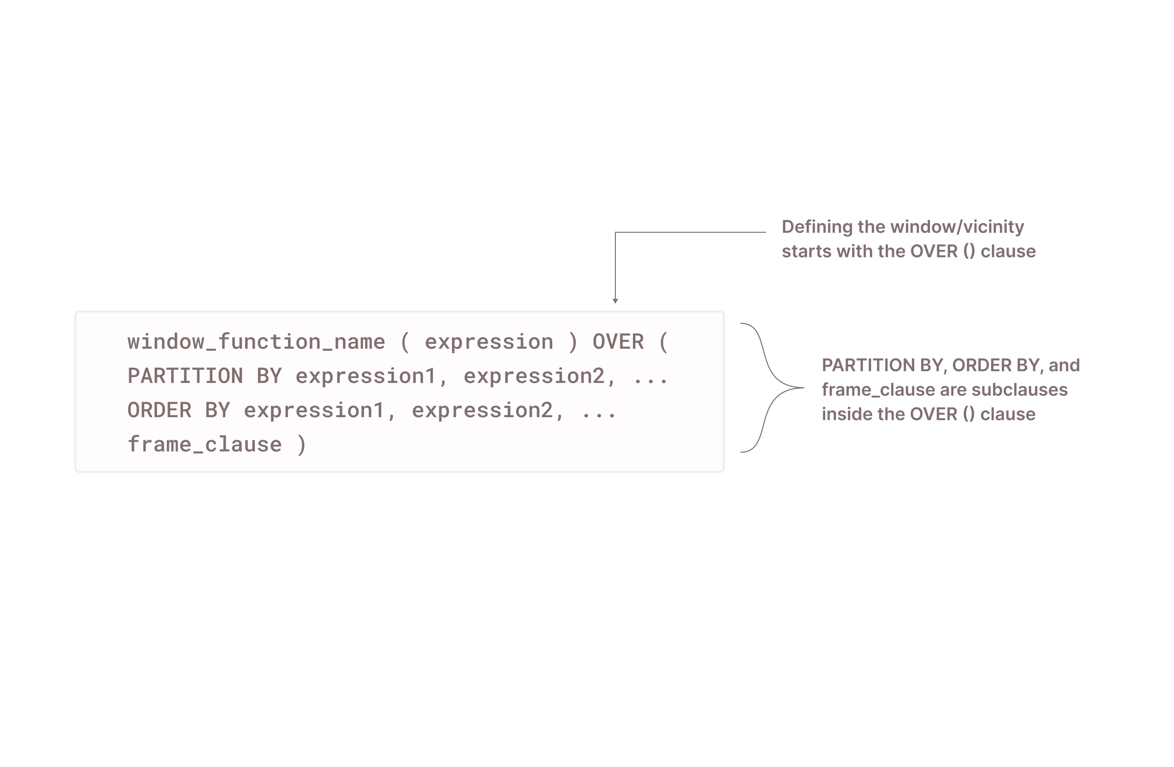
In window functions, row vicinity/window is determined using the PARTITION BY clause, ORDER BY clause, and frame_clause.

First, partitioning is used to divide query results into partitions. Imagine a scenario of a housing prices table with three columns: Country, Region, and Price. The PARTITION BY clause will divide the pricing data into partitions by country or by region. Second, the concept of row vicinity depends on the row ordering. If there is no well-defined order of the rows using the ORDER BY clause, the vicinity will be non-deterministic. 

Finally, the frame_clause determines the set of rows (the window/vicinity) that the window function includes in its calculation for each row in a partition. 

There are three types of frame clauses:

1. ROWS clause: Vicinity computation based on the physical offset of rows from the current row, measured in a specific number of rows preceding or following it.
2. RANGE clause: Vicinity computation based on the logical value in the ORDER BY expression for the current row. 
3. GROUPS clause: Vicinity computation based on the number of peer groups preceding or following the current row’s peer group.

‍Note: When the OVER()clause is used with an empty parenthesis, it means that the window function will consider the entire table as a single partition. In that scenario, row ordering is not required.

Window functions outperform traditional SQL by executing analytics directly at the database level, thereby avoiding the performance overhead of processing them at the application level. 

There are three common use cases of these window functions:

1. Aggregate functions: To calculate aggregations, including the average, count, maximum, minimum, and total sum across each window or partition (e.g., AVG(), MAX(), MIN(), SUM(), COUNT())
2. Ranking functions: To rank rows within a partition (e.g., ROW_NUMBER(), RANK(), DENSE_RANK(), PERCENT_RANK(), NTILE())
3. Value functions: To compare values between rows within a partition (e.g., LAG(), LEAD(), FIRST_VALUE(), LAST_VALUE(), NTH_VALUE())

Recursive Queries and Common Table Expressions (CTEs)

Unlike general-purpose programming languages, SQL is designed to terminate regardless of the size of the input tables. 

Recursive common table expressions (CTEs) offer SQL the ability to infinitely loop during execution. Recursive CTEs in SQL start with the WITH RECURSIVE clause and can be referenced multiple times, giving them the ability to reference themselves within the main query.

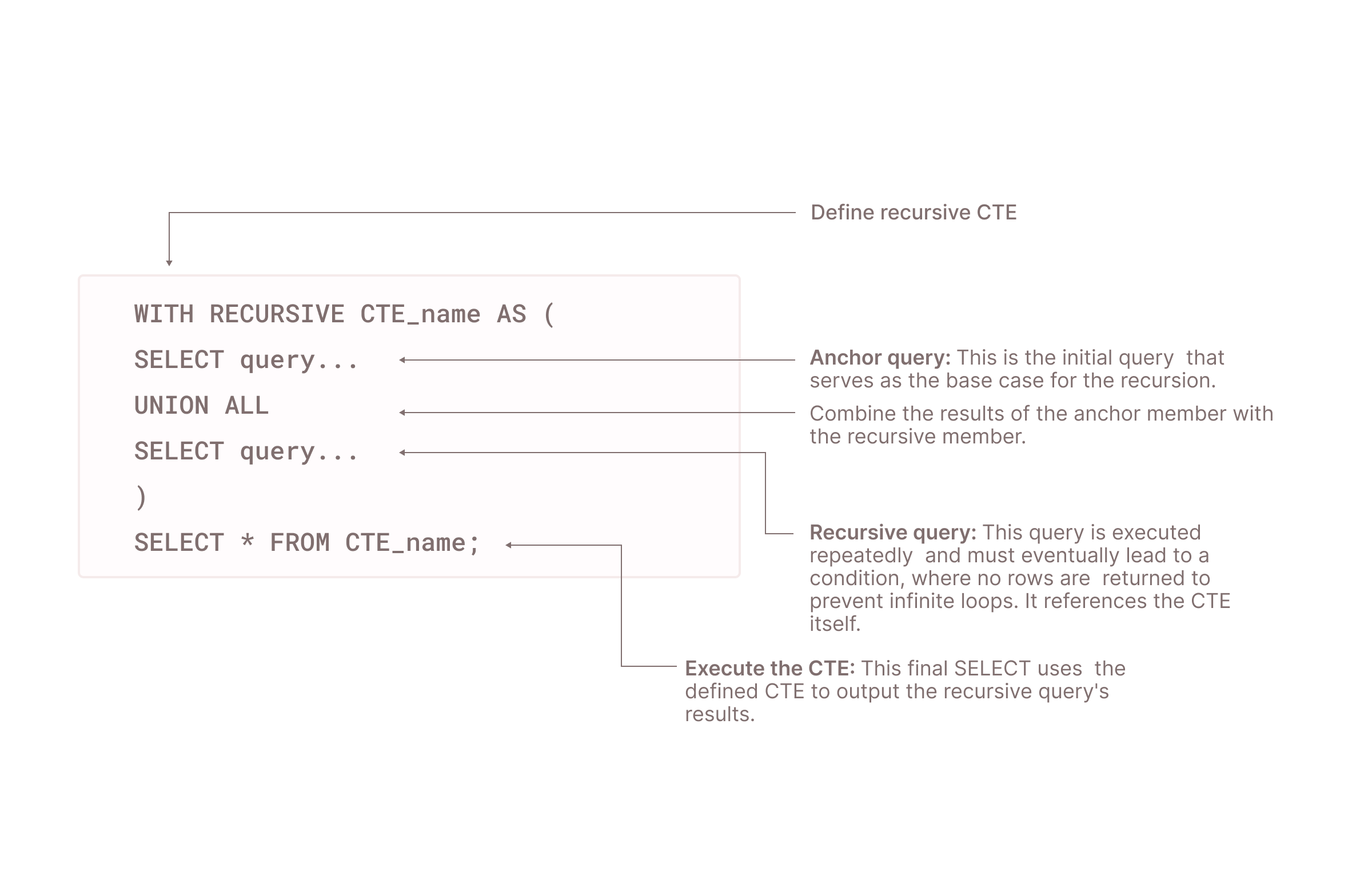
As shown above, recursive CTE execution involves multiple steps:

• Using the WITH RECURSIVE clause, the recursive CTE gets initialized. CTE_name is a placeholder for whatever name you give the CTE.
• The anchor query is executed only once at the start of the recursion. The output of this base query becomes the input for the recursive query, which you will define later.
• Recursive query references the CTE_name itself, which is what makes the query recursive. It must have a joining condition or a logical progression that moves towards a base case to ensure the recursion terminates.
• UNION ALL combines the results from an anchor query as well as a recursive query to preserve duplicates.
• Finally, SELECT * FROM CTE_name; executes the CTE and shows the output of the recursive CTE.

Let’s discuss an example to further understand the syntax and flow of this execution using the same data table discussed in Figure 2. 

Example Scenario

Imagine having a recursive CTE called DatewiseTotal that starts by aggregating financial records by date for the HR department, beginning with the earliest record:

WITH RECURSIVE DatewiseTotal AS (
  SELECT id, date, department, amount
  FROM financial_data
  WHERE department = 'HR' AND date = (SELECT MIN(date) FROM financial_data WHERE department = 'HR')

  UNION ALL

  SELECT fd.id, fd.date, fd.department, fd.amount + dt.amount
  FROM financial_data fd
  JOIN DatewiseTotal dt ON fd.date = (SELECT MIN(date) FROM financial_data WHERE date > dt.date AND department = 'HR')
  WHERE fd.department = 'HR'
)

SELECT * FROM DatewiseTotal ORDER BY date;

Initially, the WITH RECURSIVE clause declares the DatewiseTotal, using a SELECT statement to define the base case, which selects the earliest date available for the HR department. This is the entry point for the recursive accumulation of amounts. 

In each recursive iteration, a JOIN operation is conducted, which links the current totals in DatewiseTotal with the next chronological record from the financial_data table. 

The recursive query continues to execute, adding the amount from each succeeding record to the cumulative total previously calculated. This step-by-step aggregation persists day by day, compiling the amounts until there are no further dates to process, which effectively terminates the recursion. 

Finally, SELECT * FROM DatewiseTotal ORDER BY date; prompts the query to output the accumulated totals in chronological order, as seen in Figure 6 below.

SQL Query Optimization Techniques

SQL optimization relies on a set of practices for improving query performance, such as reducing query execution time and preventing excessive use of system resources. These techniques require a high-level understanding of how SQL performs calculations and what factors are within your control. 

For example, query runtime increases with table size, the number of joins, and the number of aggregations; therefore, optimum performance can be achieved by correctly manipulating these factors. 

Among the many techniques in use today, the following are some of the most important for tuning query performance.

Breaking Down Complex Queries 

Smaller, more modular queries are a strategic approach for optimizing SQL query performance. This method can enhance efficiency, manageability, and even readability by reducing complexity while improving readability, maintenance, and caching efficiency.

Reducing Query Execution Time 

An optimized query must retrieve only the necessary records from a database, thereby lowering execution time. Queries like SELECT *, SELECT DISTINCT, and cartesian joins with WHERE clauses require more computation. Avoiding SELECT * and SELECT DISTINCT, and using INNER JOIN instead of WHERE. can significantly reduce computation time.

Indexing 

Indexes allow fast retrieval of data by eliminating the need to look through every row in a database table. In SQL, there are two types of indexing: clustered and nonclustered. A clustered index stores rows physically on the disk in the order of the index itself, whereas a non-clustered index maintains a separate list of pointers that refer back to the physical rows in the table. 

Well-defined indexes can reduce disk I/O operations and use fewer system resources. By using index tuning tools such as Database Engine Tuning Advisor (DTA), the MySQL query optimizer, and Oracle SQL Tuning Advisor, you can provide recommendations to add, modify, or remove indexes in your SQL database.

Creating and Monitoring Query Execution Plans 

RDBMS query execution plans provide the flow of how a database engine processes a query. It details the operations, such as joins, sorts, and scans, that the database performs to retrieve the data. By analyzing these, data engineers can spot inefficiencies such as full table scans, suboptimal join orders, or missing indexes. 

This visibility allows for targeted optimizations, such as restructuring the query, adding indexes, or modifying database schema to ensure that the database engine can execute the query in the most efficient way possible.

Optimizing Database Schema

In relational databases, schema provides the logical structure of database objects, for example, tables, columns, and views. Good schema design can significantly increase query performance. 

MySQL documentation has some best practices for designing your database. Open-source tools like SeeQR can also analyze the efficiency of schema to make better-informed architectural decisions.

Handling Complex Data Transformations

Data transformation is an everyday requirement in data engineering. Building ETL/ELT pipelines for data warehouses requires advanced schema transformation capabilities from relational modeling to dimensional modeling. Tools such as dbt and Apache Airflow are created specifically to perform the transformation phase in ELT/ETL workflows.

‍

Below are some best practices for you to follow for complex data transformations, allowing you to ingest and query your data with low latency and scalability.

Joining Multiple Tables Efficiently

Common techniques for joining multiple tables include:

• Structure joins so that a large table joins with a smaller table to optimize query execution.
• Avoid CROSS JOIN; this gives you the cartesian product of rows from joined tables, which can be resource-intensive; implement INNER JOIN and OUTER JOIN for more control over the result set.
• Index foreign keys to accelerate join operations, as the database engine can quickly locate the join columns.

Pivoting and Unpivoting Data for Analysis

PIVOT transforms SQL tables by rotating rows into columns, whereas UNPIVOT is used to reverse that process. These transformations help with reporting when you need to compare metrics across categories or periods.

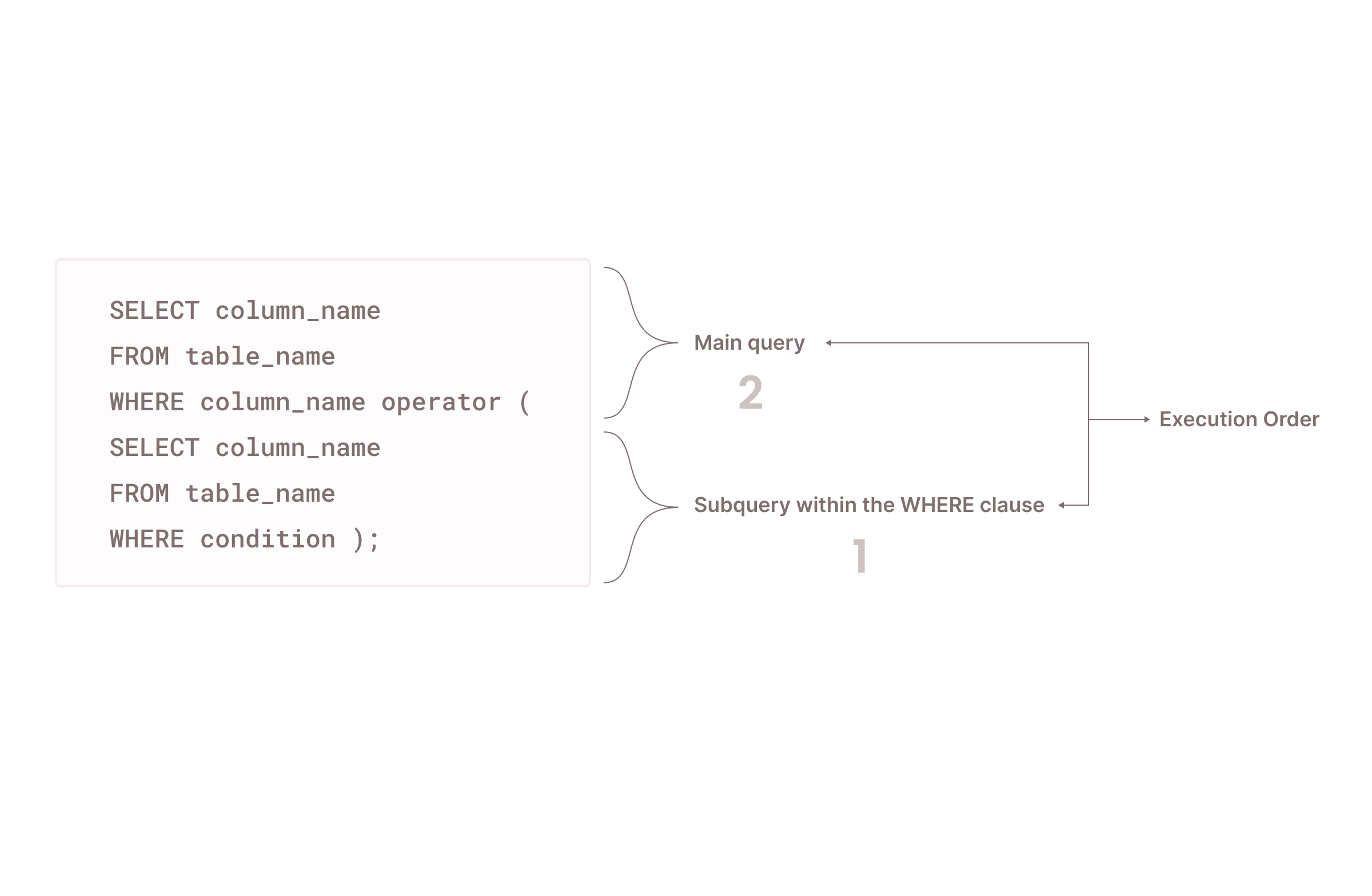
Working with Nested Queries/Subqueries Effectively

Subqueries are SQL queries nested or embedded within another SQL query. They simplify complex business logic by dividing it into smaller, more manageable queries. However, you must use subqueries carefully, as there are scenarios where subqueries can slow down the execution time (e.g., when dealing with large data sets and correlated subqueries).

Advanced Error Handling and Debugging

Like any other programming language, SQL error handling and debugging must start with exception handling. However, SQL has exception-handling syntax that is vendor-specific. For example, you can use TRY…CATCH blocks only in SQL servers, whereas MySQL uses handler declarations within stored procedures to handle exceptions. 

Postgress SQL and Oracle have different approaches for exception handling with BEGIN...EXCEPTION...END blocks. Also, it’s recommended that custom error messages be defined for improved diagnostics and debugging.

Logging and monitoring can also help with faster debugging. This involves tracking information such as query execution, transaction operations, and system health. Users can leverage vendor-specific built-in logging and monitoring features or rely on the many third-party open-source solutions, including Prometheus, Grafana, Adminer, HeidiSQL, Flyway, DBeaver, etc.

Conclusion

Advanced SQL queries combine powerful concepts such as window functions, recursive CTEs, and efficient indexing to elevate query performance and streamline complex data transformations. When used properly, these techniques help you optimize execution times, maintain cleaner data pipelines, and stay adaptable to changing requirements.

As a data engineer, honing these skills will not only increase your ability to solve intricate problems but also ensure that your data architectures remain robust over the long term. To truly master these methods, regular practice with real-world data sets is essential. Experiment with different optimization tricks, pay close attention to execution plans, and fine-tune indexes based on your findings. 

As you refine your approach, drop any feedback or your own favorite SQL tricks to our Firebolt LinkedIn handle.